

Optimizing Your Perl
Is your Perl program taking too long to run? This might be because you’ve chosen a data structure or algorithm that takes a long time to run. By rethinking how you’ve implemented a function, you might be able to realize huge gains in speed.
Some Simple Complexity Theory
Before we can talk about speeding up something, we need a way to describe how long something takes. Because we’re talking about algorithms that may have varying amounts of input, the actual “time” to do something isn’t conclusive. Computer scientists and mathematicians use a system called big-O notation to describe the order of magnitude of how long something will take. Big-O notation represents a worst-case analysis. There are other notations to represent the magnitude of minimum and actual runtimes.
Don’t let the talk of computer scientists and mathematicians scare you. The next few paragraphs talk about a way to describe the difference between orders of magnitude such as a second, minute, hour or day. Or 1, 10, 100 and 1,000. You don’t need to know any fancy or scary math to understand it.
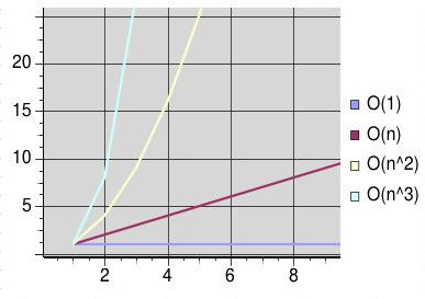
It’s simple. If the runtime of a function is constant, then this is written as O(1). (Note the capital or “big” O.) Constant means that no matter how much data is processed, (i.e., how much input there is) the time doesn’t change.
If the runtime is directly related to the amount of input (a.k.a. linear), then this is O(n). If there is twice as much input, then the algorithm will take twice as long to run. Some functions are O(n^2) (quadratic) or O(n^3) (cubic) or even worse.
Because we are only looking at orders of magnitude (is the operation going to take one minute or one hour) we can ignore constant factors and smaller terms. O(2n) and O(n) are equivalent. As are O(n+1) and O(n) or O(n^2+n) and O(n^2). The smaller term is insignificant compared to the larger.
There are rules for analyzing code and determining its big-O, but the simplest way is to look at how many times you iterate over the data. if you don’t iterate, then it’s O(1). If you iterate over it once, then it’s O(n). If you have two nested loops, then it’s probably O(n^2).
Example #1: Graphing
I developed a new graph module for a project at my day job, because the existing one was overkill, yet did not support a feature I needed. It was easy to implement and worked very well, until the graph got very big. I needed flattened subgraphs to do dependency checks, but it was taking more than two minutes to compute (on a 1Ghz P3) for a 1,000 node graph. I needed the computation to be much faster, or my users would get mad.
My initial Graph module looked like this. (Simplified to only show relevant parts.)
 package Graph; # for Directed Graphs
 use strict;
 sub new {
  my $this = { edges => [],
               vertices => {} };
  bless $this, "Graph";
 }
 sub add_edge { # from x to y
  my ($this,$x,$y) = @_;
  $this->{vertices}{$x}++;
  $this->{vertices}{$y}++;
  push @{$this->{edges}},[$x=>$y];
 }
 sub in_edges {
  my ($this,$v) = @_;
  grep { $_->[1] eq $v } @{$this->{edges}};
 }
The add_edge method is O(1) because it will always take the same amount of time no matter how many nodes/edges are in the graph. The in_edges method is O(n) because it has to iterate over each edge in the graph. (The iteration is “inside” the grep.)
The problematic section of the code looked like this:
 sub flat_subgraph {
    my ($graph,$start) = @_;
    my %seen;
    my @worklist = ($start);
    while (@worklist) {
      my $x = shift @worklist;
      push @worklist, $graph->in_edges($x)
         unless $seen{$x}++;
    }
    return keys %seen;
 }
And I actually needed to do that for multiple vertices;
  my %dependencies;
  for (keys %{$graph->{vertices}}) {
   $dependencies{$_} = [ flat_subgraph( $graph, $_ ) ];
  }
This would make the entire flattening operation O(n^3). ( The dependency loop is O(n), flat_subgraph is effectively O(n), and in_edges is O(n)). That means that it takes much longer to compute as the Graph becomes bigger. (Imagine a curve with the following values: 1,8,27,64…, that’s the curve of relative times.)
Caching
With my users expecting instant feedback, something had to be done. The first thing I tried was to cache the in_edges computation.
 sub in_edges {
  my ($this,$v) = @_;
  if (exists $this->{cache}{in_edges}{$v}) {
      return @{$this->{cache}{in_edges}{$v}};
  } else {
    my @t = grep { $_->[1] eq $v } @{$this->{edges}};
    $this->{cache}{in_edges}{$v} = [@t];
    return @t;
   }
 }
This helped, but not as much as I had hoped. The in_edges calculation was still expensive when it wasn’t cached. It’s still O(n) in the worst case, but becomes O(1) when cached. On average, that means the entire flattening operation is somewhere between O(n^2) and O(n^3), which is still potentially slow.
In situations where the same functions are called with the same arguments, caching can be useful. Mark-Jason Dominus has written a module called Memoize, which makes it easy to write caching functions. See his Web site http://perl.plover.com/MiniMemoize/ for more information.
Change the Structure
The next thing I tried was to change the Graph data structure. When I originally designed it, my goal was simplicity, not necessarily speed. Now speed was becoming important and I had to make changes.
I modified graph so that in_edges were calculated when the new edge was being added.
 package Graph; # for Directed Graphs
 use strict;
 sub new {
  my $this = { edges => [],
               vertices => {},
               in_edges => {} };
  bless $this, "Graph";
 }
 sub add_edge { # from x to y
  my ($this,$x,$y) = @_;
  $this->{vertices}{$x}++;
  $this->{vertices}{$y}++;
  push @{$this->{in_edges}{$y}}, $x;
  push @{$this->{edges}},[$x=>$y];
 }
 sub in_edges {
  my ($this,$v) = @_;
  return @{$this->{in_edges}{$v}};
 }
add_edge remains O(1) - it still executes in a constant time. in_edges is O(1) as well now; its runtime will not vary based on the number of edges.
This was the solution I needed, getting a full flattening down from more than four minutes to only six seconds.
The Importance of Good Interfaces
One of the things that made this fiddling possible was a good design for the Graph module’s interface. The interface hid all the details of the internals from me, so that different implementations could be plugged in. (This is actually how I did the testing, I had a regular Graph, a Graph::Cached, and a Graph::Fast. Once I decided that I liked Graph::Fast the best, I renamed it to just Graph.)
I’m glad I designed Graph the way I did. I put simplicity and design first. There is a phrase you might have heard: “Premature optimization is the root of all evil.” If I had optimized the Graph module first, then I might have ended up with more complicated code that didn’t work in all cases. My initial cut of Graph was slow, but worked consistently. Optimization happened later, after I had a baseline I could return to, to guarantee proper operation.
Example #2: Duplicate Message Filter
You don’t always need to try and optimize code to the fullest extent. Optimizing code takes your time and energy, and it isn’t always worth it. If you spend two days to shave two seconds off a program, then it’s probably not worth it. (Unless of course, that program is running hundreds of times each day.) If a program is “fast enough”, then making it faster isn’t worth it.
Our second example is a duplicate message filter for e-mail. This filter is useful when you receive cc’s of messages also sent to mailing lists you are on, but you don’t want to see both.
The general idea behind this filter is simple.
skip $message if seen $message->id;
It’s only the seen function that interests us. It searches some form of cache of id’s. How we implement it can have a large effect on the speed of our mailfilter. (For more information on filtering mail with perl, take a look at Mail::Audit.)
The two most obvious methods that come to mind for implementing seen are a simple linear search (O(n)) or the use of a persistent database/hash table to do the lookup. O(1). I’ll ignore the cost of maintaining the database, eliminating old Message-Id’s, etc.
A linear approach writes out the message id’s with some sort of separator. Some programs use null bytes, others use newlines.
The database/hash method stores the message id’s in a binary database like a DBM or Berkeley DB file. At the expense of using more disk space, lookups are generally faster.
But - there’s one more factor to take into account - overhead. The linear search has little overhead, while the DB file has a large overhead. (Overhead here means time to open the file and initialize the appropriate data structures.)
 TABLE: Comparison

  Records | Comment
  -----------------
    100   | linear is 415% faster
    250   | linear is 430% faster
    500   | hash is 350% faster
   1000   | hash is 690% faster
I performed a set of timings with a rough example implementation on my P2/400, and received the above results. The hash lookup speeds remained constant, while the linear lookup dropped off rapidly after 250 items in the cache.
Returning to the big picture, we need to take our message-id cache size into account when determining the method to use. For this kind of cache, there’s usually not a reason to keep a huge amount of entries around, only two or three days worth should catch most duplicate messages. (And probably even one day’s worth in most cases.)
For this problem, an O(1) solution is possible, but the constant time it takes might be higher than an O(n) solution. Both cases are trivial to implement, but in some situations it will be difficult to implement O(1) - and not worth it either.
Conclusion
Perl is a powerful language, but it doesn’t prevent the programmer from making poor decisions and shooting him/herself in the foot. One mistake is to choose the wrong data structure or algorithm for the job. By using a little bit of complexity theory, it’s possible to optimize your code and get huge speed gains.
I’ve only touched the surface of big-O notation and complexity theory. It’s a highly researched topic that delves into the deep dark corners of math and computers. But, hopefully there’s enough here to give you a basic tool set.
As the second example showed, you don’t necessarily want to spend too much time thinking about optimization. Over-optimization isn’t always worth it.
For More Information
http://www.google.com/search?q=big-O+complexity
Introduction to the Theory of Computation
Part Three of Sipser, Michael. “Introduction to the Theory of Computation”. PWS Publishing Company. Boston, MA. 1997.
Algorithms and Complexity, Internet Edition
http://www.cis.upenn.edu/~wilf/AlgComp3.html
Special Thanks
Walt Mankowski
Tags
Feedback
Something wrong with this article? Help us out by opening an issue or pull request on GitHub

